A theoretical approach to cardioid subwoofers (with practical consequences)
The use of cardioid subwoofers in large sound reinforcement systems is common practice today, thanks to the availability of digital signal processors. Many loudspeaker system manufacturers offer presets that users can put in operation without having to dwell in the theoretical aspects of this technique. However, this technique is well-documented in its principle, but not in regard to its limitations and caveats. This paper intends to dig a little deeper, without having to resort to a lot of mathematics.
The basic principle(s)
When questioned about the operating principle of cardioid subwoofers, many sound operators describe only one set-up, and very often add that the delay value that is used in the electronic delay line must be calculated in accordance with some "wavelength of the system". The next paragraph shows that the delay setting depends only on the physical placement of the system.
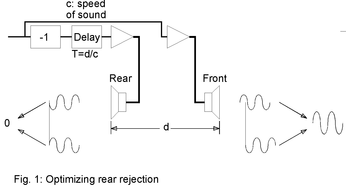
Optimizing rear rejection The basic train of thought is that, by introducing in the rear space an out-of-phase image of the spillage from the front, the rear wave would be cancelled. A practical implementation is shown on Fig. 1. The rear subwoofer is fed with an out-of-phase version of the front signal, the electronic delay is adjusted to achieve exactly the same delay as the time the front wave takes to reach the rear space.
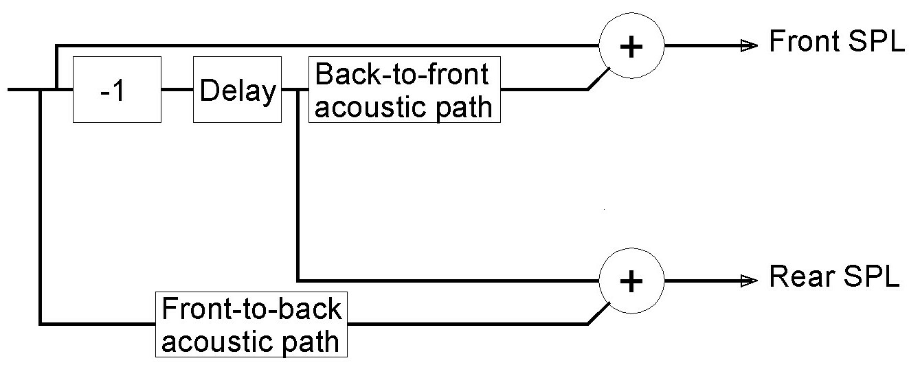
Many users are satisfied with this description and think there is nothing else to it. In fact, a simulation shows that, although the rear rejection is as expected, the front response of the resulting system suffers serious reduction in performance and limitations. The model used for simulation is shown in Fig. 1b.	Fig. 1b: Model of "rejection-optimized" set-up
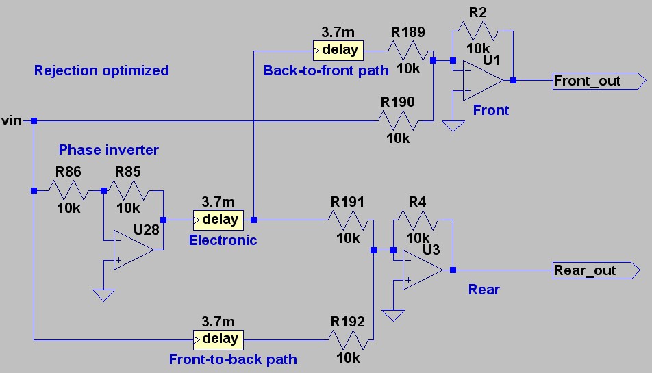
The model is then entered into a simulation software (LTSpice IV by Linear Technology). The resulting schematic diagram is shown in Fig. 1c. In this example, and in many of the following, we have set the distance at 1.27m (50"), corresponding to 3,7ms of delay, typical of the array of Fig. 6	Fig. 1c: Diagram of "rejection-optimized" set-up
The resulting frequency responses of the front and rear SPL are plotted in Fig. 1d. One can see that the optimum rejection goal is achieved, but at the expense of the front response which shows a lack of efficiency at VLF (+1dB coupling at 30Hz, instead of the expected 6dB), and a severe notch effect at 135Hz. In fact, due to a number of acoustic interferences, it is impossible to achieve the expected rejection figures. Practically, achieving 12dB of rejection is a commandable feat.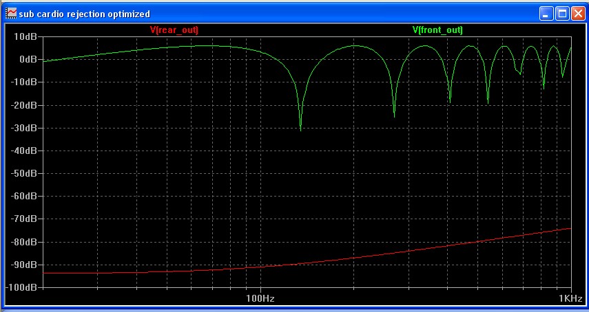	Fig. 1d: Response of "rejection-optimized" set-up Green: front response Red: rear response
Optimizing the front wave
Taking the problem by the other side, the idea is processing the rear speaker signal insuch a way that its spillage into the front zone comes exactly in phase with the front signal. Since the signal from the rear subwoofer is dealyed by the back-to-front path, it ensues that the front signal must be delayed. This could appear as an unwelcome feature, as sound engineers are very reluctant to add delay in their set-ups, but in fact, very often, and mainly for practical reasons, subwoofers are mounted in front of the main speakers, so that should not be a big issue. A practical implementation is shown on Fig. 2.
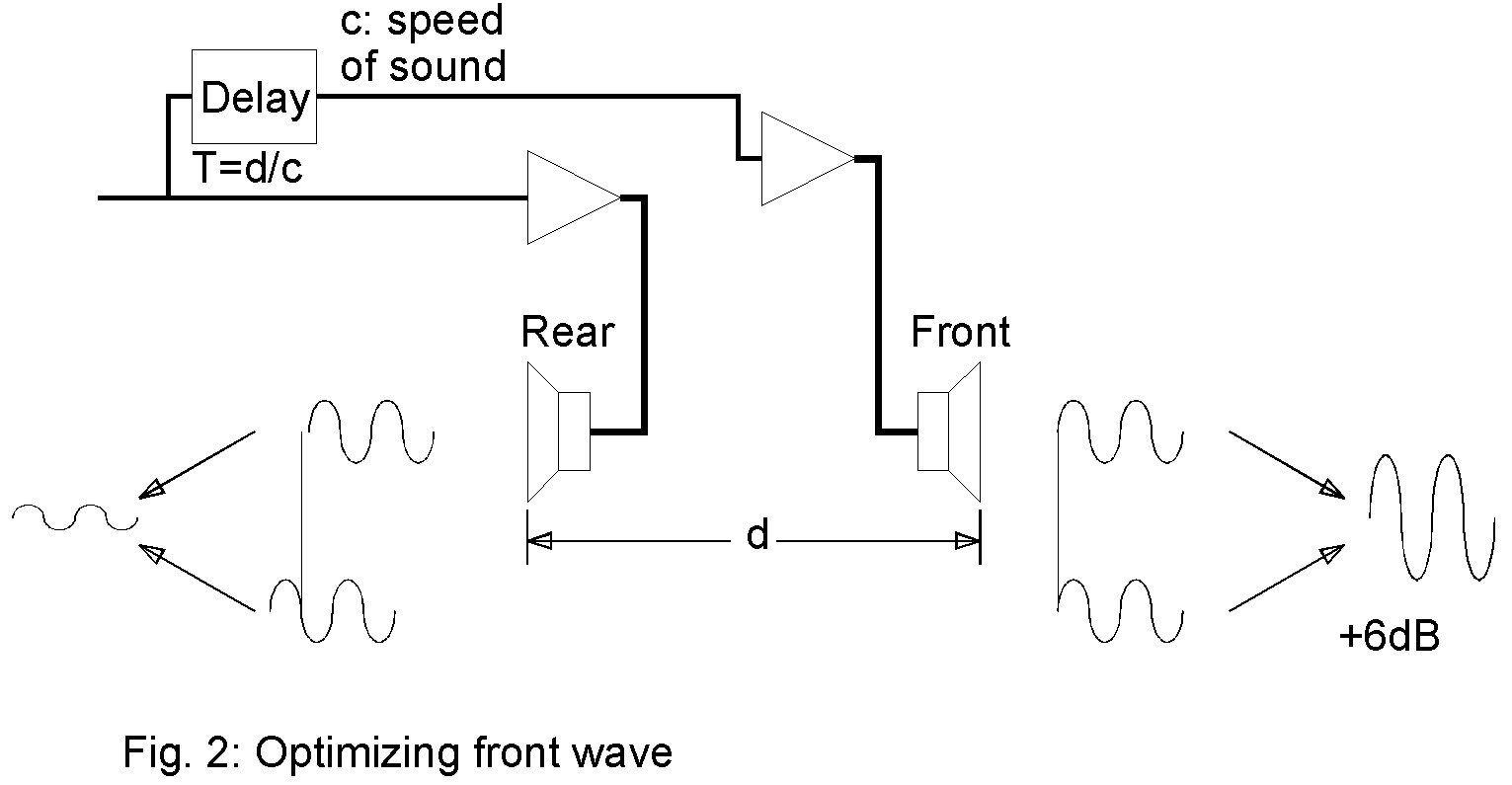
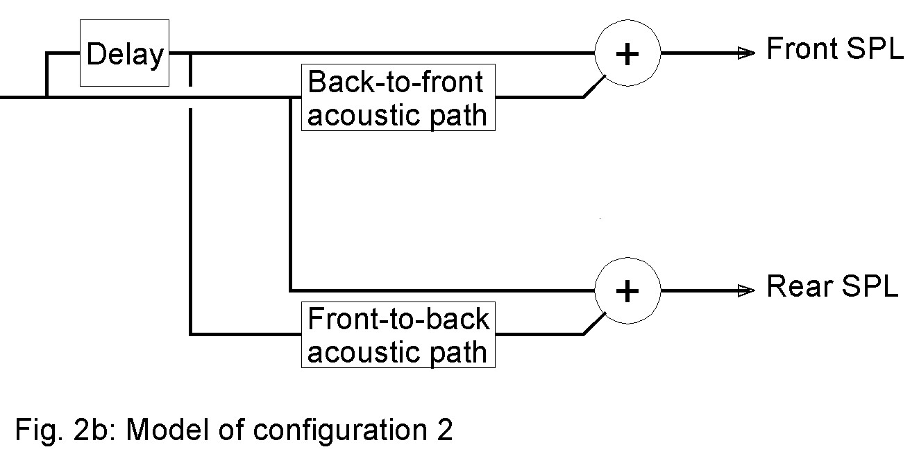
The front subwoofer is fed with a delayed version of the rear signal, the electronic delay is adjusted to achieve exactly the same delay as the time the rear wave takes to reach the front space. Now it is time to check the performance of this configuration. The model used for simulation is shown in Fig. 2b.
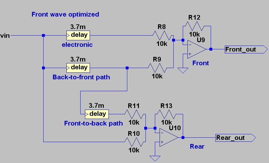
The resulting schematic diagram is shown in Fig. 2c.	Fig. 2c: Diagram of "front-wave-optimized" set-up
The resulting frequency responses of the front and rear SPL are plotted in Fig. 2d. As expected, the front response now shows perfect coupling at +6dB, but the rear rejection is not as good as it used to be. Or is it? In fact the rejection at VLF is not very good, with only about 1dB at 20Hz, 4dB at 30Hz and 7dB at 40Hz. At 100Hz, which is the limit of operation of most subwoofers in large installations, the rejection is about 8dB. So apparently this configuration does not look very impressive. However, let's have a look at the frequencies between 45Hz and 80Hz, which is where most of the subwoofers activity is concentrated. The rejection is always superior to 10dB, with a whopping notch at 65Hz, which is probably the most problematic frequency in terms of stage pollution.	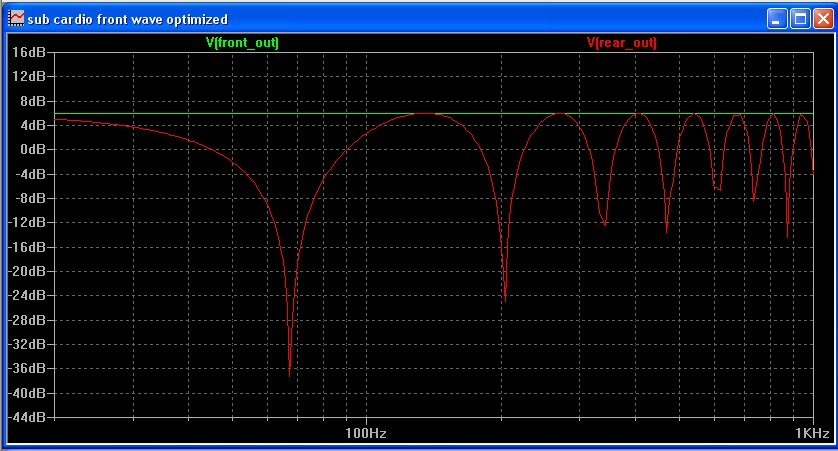Fig. 2d: Response of "front-wave-optimized" set-up Green: front response Red: rear response
As we shall see, this set-up is the basis of the end-fire arrays, which are the subject of the next paragraph.
The end fire array
The end-fire array is just an extension of the preceding system, using a larger number of elements. A practical implementation, using three subwoofers, is shown on Fig. 3.
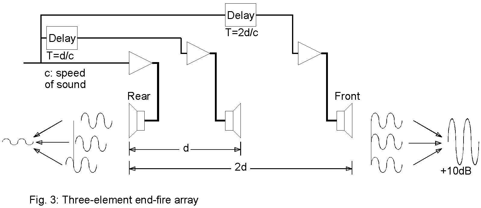
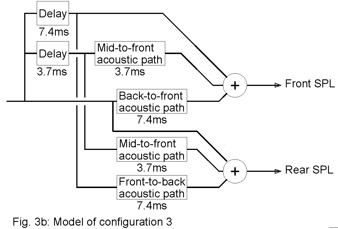
The front subwoofer is fed via an electronic delay tuned to the length of the back-to-front acoustic path. The mid subwoofer is fed via an electronic delay tuned to the length of the mid-to-front acoustic path. The model used for simulation is shown in Fig. 3b.
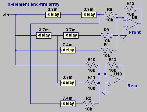
The resulting schematic diagram is shown in Fig. 3c.	Fig. 3c: Diagram of 3-element end-fire array
The resulting frequency responses of the front and rear SPL are plotted in Fig. 3d. The front response shows the expected increase of about 10dB, and the rear rejection is better than 10dB in the 33Hz-100Hz frequency range, with deep notches at 45 and 90Hz.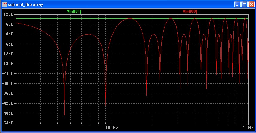	Fig. 3d: Response of 3-element end-fire array Green: front Red: rear
Because it looks promising, here are the results of a simulation of a 5-element end-fire array (Fig. 4d). Indeed the results are impressive, with 12 dB rejection in the 22Hz-110Hz frequency range. 12dB doesn't seem like a lot, but in fact, in comparison with the best practical results achieved by the "rejection-optimized" configuration, it is probably the best solution, provided there is enough depth to install 5 rows of subwoofers.	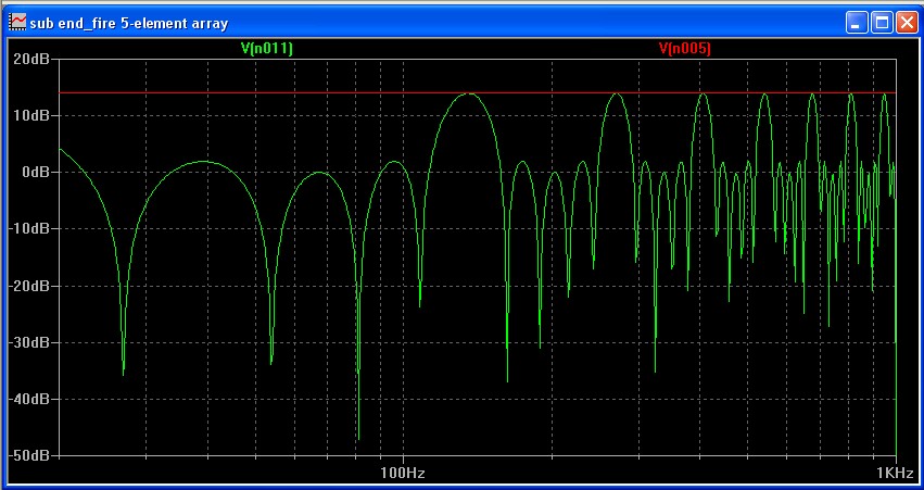Fig. 4d: Response of 5-element end-fire array Red: front Green: rear
An interesting variant: the hypercardioid pattern
The "rejection-optimized" configuration is characterized by a good rejection of sound in the rear axis of the array, which is not always the ultimate goal. In fact, the actual goal is reducing stage pollution, and very often, the speakers are located on the sides of the stage. So it becomes evident that the direction of maximum rejection should be directed towards the stage. One of the possible solutions is to orient the subwoofer arrays radially in reference to the stage. The obvious consequence is that the main front axis would also be divergent, which may not be to the likings of the SE and the public. 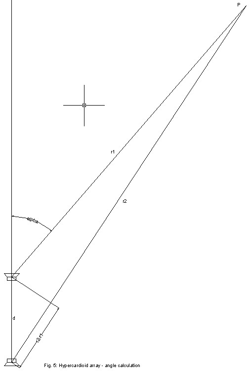The operation of the array can be very easily modified to offer a hypercardioid pattern. Such a pattern has two null rear-axis, at the detriment of on-axis rear rejection. Since we want to do with as little math as we can, let's consider the case where the electronic delay were zero. The subs would be driven by out-of-polarity signals. It ensues that total cancellation would occur in any postion that is at the same distnace from both subs. The totality of these locations (mathematically the locus) is a plane passes at mid-distance between subs and that is perpendicular to the axis. In fact, this configuration is very well known as a dipole, exhibiting the equally well known "figure-of-eight" directivity pattern. Rejection is optimized on the sides of the array, which may be a good thing, but the front-wave efficiency is 6dB down and the rear-wave is equal to the front. The angle is given by the formula cos alpha = T/delta T being the electronic delay, delta the time equivalent to the distance between subs, converted using the formula delta = d/c It is easy to demonstrate that, except for very short distances, the locus of optimum rejection is a cone with a projected angle of alpha x 2. This is true for free-standing subwoofers. When the subs are floor-mounted, which is often the case, a distortion of the 3D pattern occurs, but still the basic calculation works. In conclusion, reducing the delay steers the pattern from true-cardioid (180° rejection) towards figure-8 (90° rejection) via all variations of hypercradioid. The simplicity of this process makes experimentation very easy: simply variyng the delay controls the aiming of the rejection zone.
How do parameters influence the performance?
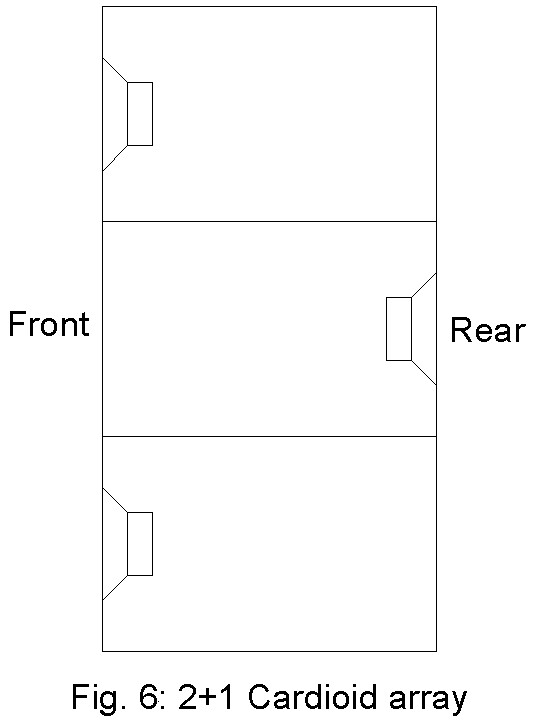
Now is the time to evaluate the influence of the different parameters in regard to the expected performance. As we've just seen before, modifying the delay time provides useful control of the directivity pattern. Let's evaluate the importance of the rear-to-front power ratio. Until now, we have considered that the power of the rear sub was the same as the front one. In view of the quite-common recommendation of many speaker manufacturers to establish a 2:1 ratio, as shown in Fig. 6, let's examine the consequences. In order to do so, we use our good old simulation package, and we drive the rear speaker with 6dB less signal, which gives the response graph of Fig. 6b.
We can see that the front SPL is reduced by 2,5dB, which was to be expected because the overall power has decreased, but also that the rejection has drastically diminished, being now a mere 9dB in the 70-90Hz range. How can this be acceptable? First, let's be realistic. What is the point in achieving 20 or 30 dB rejection in the 30-100Hz range if there is a lot of spillage from the low-mids? Achieving a practical rejection of 15dB is a feat! Second, we have assumed perfectly omnidirectional subs. In fact, they aren't. Their size confer subwoofers some directional properties. With 700mm (27") height, a subwoofer shows -3dB rear rejection at 120Hz (700mm is the quarter-wavelength at 120Hz). At 60Hz, it shows about 1dB rear rejection, which is not much and not terribly significant. But when the subwoofers are assembled in a three-high array, the -3dB directivity goes lower. In fact there, the width is the limiting factor. Most subwoofers are about 1.2m wide, which makes the 3dB point down to 70 Hz, which is the frequency zone which we want to improve. If we enter that in our simulation package, we obtain the graph in Fig. 6c. Now the rejection is about 9dB in the 50Hz-80Hz range, which seems an acceptable performance. Now, how does one choose the distance between sources? A very important aspect of this study is the fact that with the "rejection-optimized" configuration, the VLF response shows a significant drop. It can be easily demonstrated that the effect is the same as a 1st-order (6dB/octave) high-pass filter with a cut-off frequency which wavelength is 4 times the distance between subs, or which period is 4 times the delay. In our case, 4x3,7ms => F = 67,5 Hz. As well, the upper limit of operation is directly related to the distance separating the front and rear sources. The notch appears at twice the cut-off frequency, 135 Hz in our example. Basically a "rejection-optimized" array has a very restricted range of about one octave. It seems that most operators are content with that, the benefit of reducing stage pollution largely exceeding the drawback of restricted bandwidth.	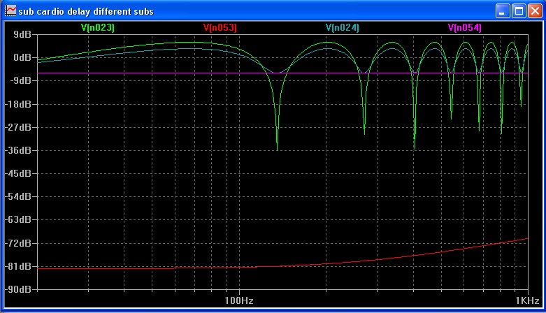Fig. 6b Green: Front response with full-power on both subs Red: Rear response with full-power on both subs Cyan: Front response with half-power on rear sub Magenta: Rear response with half-power on rear sub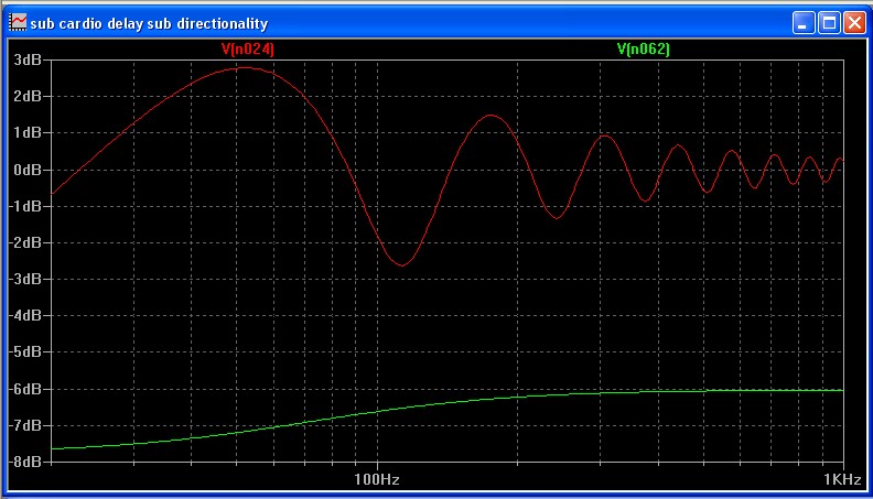 Fig. 6c: Simulation taking "natural" directivity into account.
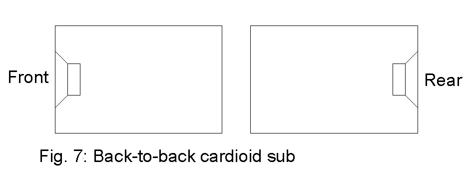
Let's analyse the consequences of placing the subs further appart, as is the case when set up back-to-back, according to Fig. 7.
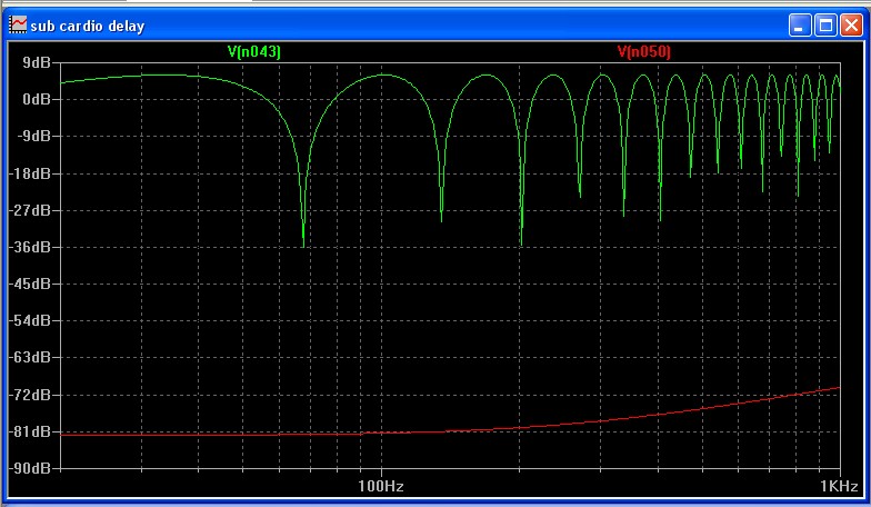
The delay has now doubled, to 7,4ms, and the simulation results can be seen on the graph at Fig. 7b. The VLF response has improved notiveably (the LF cut-off is now 34Hz) and the upper limit is still 135Hz, but there's a BIG notch at 67Hz!	Fig. 7b. Response of back-to-back sub array Green: front Red: rear
It looks like this is completely unusable, but this set-up, used in conjunction with the array of Fig. 6, which has its maximum efficiency at 67Hz, could be a perfect complement. Such a combined system is represented in Fig. 8.
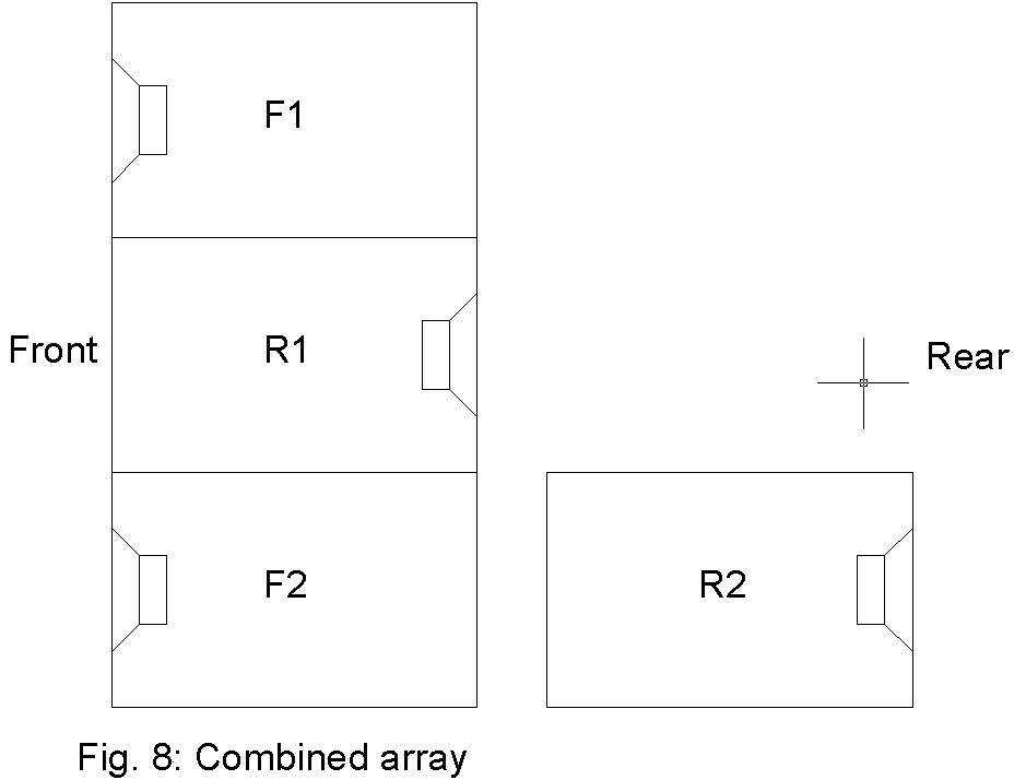
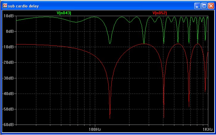
Simulation of such a combination can be seen on Fig. 8b. This system is flat within +/-1dB in the range 22-110Hz and the rejection is close to 20dB!	Fig. 8b: Response of combined array Green: front Red: rear
Conclusion
Until now, sound engineers have used ready-made receipes for their cardioid subwoofer experimentations. These theoretical explorations will help them in the understanding of the mechanisms involved, and encourage them to experiment. On a theoretical point of view, the end-fire array is less flawed than the "rejection-optimized" one, but it is impractical in many cases, so it seems that the latter will still be used in a majority of cases. However, the combined array seems to overcome most problems, whilst being usable in most situations. A number of real life issues have not been taken into account, such as the effects of reflections, but the practical implications of theory are nevertheless valid.
Copyright JLM 2011